
This version of the ISM ice sheet model runs interactively on your browser while you clobber it by dragging the global temperature up and down, or dosing it with CO2. You can "replay" the forcing history from one run to drive another run with different characteristics, for direct comparison.
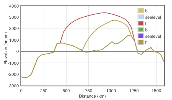 |  |
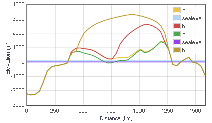
The red and beige curves show the elevation of the Greenland ice
sheet after considerable CO2 forcing, for cases with and
without Basal Sliding. The lower three entries in the legend are for
the Control simulation (previously run and saved, in this case,
with basal sliding off) and the upper three are for the Live
simulation, which uses the same forcing as the Control (but now has
basal sliding turned on). The elevations are labeled h in the
legend, b is the elevation of bedrock, and sealevel is
sea level.
|
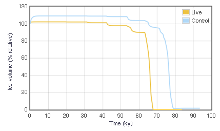
The evolution of Ice Volume though time for the Control and Live simulations.
|
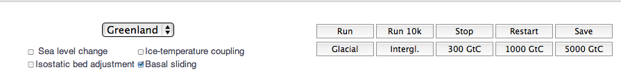
Select Greenland or Antarctica and set the model characteristics using the controls on the left. The model is set up to simulate the ice sheets along transects shown in maps here.
The click boxes enable or disable various Model settings, such as
| Sea level change | When you change the temperature, the sea level follows along, the way it did during glacial / interglacial cycles. |
| Isostatic bed adjustment | When ice melts, the decreased load allows the bedrock surface to "float up". This takes ~10,000 years. |
| Ice-temperature coupling | Allows variations in ice temperature to affect how easily it flows |
| Basal sliding | Allows the ice to slide over bedrock if it reaches the melting temperature |
The Run Control buttons are on the right. Start the modeling going by clicking Run, or you can step it forward in increments of 10,000 years using Run 10. The lower row of buttons manipulate the driving temperature of the model, taking it to either Glacial or Interglacial conditions, or by introducing a temperature anomaly that would result from release of slugs of 300, 1000, and 5000 Gt C.
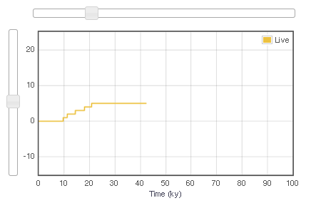 |  |
This plot shows the driving temperature
as it evolves through time. The vertical slider on the left
allows you to pull the temperature up and down as the model runs
(click Run first then drag this slider). When you save a run as a
Control, this slider disappears, because the new Live simulation will
be driven by the saved temperature history from the Control run.
The horizontal slider at the top of the plot can be used to
look back at time slices of a model run that you’ve already done, or
you can drag the model to go to a particular place in time by dragging
the slider to the right. In this shot, the model ran to about 40 kyr but the user
dialed back to see what the simulation looked like at about 20 kyr. |
Elevation plot. This plot shows the heights (elevations) of
the ice sheet, bedrock, and sea level. If you have Saved a Control
run and superimposed on it a Live run, there will be two sets of plots
superimposed, as here. The Control simulation is the lower one in the
legend, and the Live simulation is the upper set of entries. The
elevations are labeled h in the legend, b is the
elevation of bedrock, and sealevel is sea level. The Live
simulation enabled all model options. You can see the differences in
the ice thickness, the bedrock elevation (because of isostatic rebound
in Live), and sea level, between the simulations. |
|  |
The evolution of Ice Volume
though time for the Control and Live
simulations. | Other model variables, including
Ice Velocity, the Mass Balance (accumulation of net
ablation of ice), and Surface Temperature. |
To compare two model settings, do a model run with some temperature driving, then click Save Control. All the model information is saved to “background” for overlay comparison with new runs. The temperature forcing controls (vertical slider and lower level of run-control buttons) disappear, because new model runs will now be done using the same forcing as the original run had. This makes it easy to see the effect of changing model options (check boxes). Get rid of the background plot by Deleting it.
| How much CO2 emission is required to destabilize the Greenland Ice Sheet? |
| Document the sensitivity of the model to processes of basal sliding, sea level, and ice rheology. |
| How does potential fossil fuel CO2 forcing compare with glacial / interglacial forcing? |
 |
The University of Chicago 5801 South Ellis Ave Chicago IL 60637 773.702.1234 |